Ancestral state reconstruction of a trait
Source:vignettes/ancestral_state_reconstruction_of_a_trait.Rmd
ancestral_state_reconstruction_of_a_trait.RmdIntroduction
This tool’s main workhorse is the asr(), which leverages corHMM’s ancestral state reconstruction algorithm to characterize genome-influenced features’ gain, loss, and continuation across a phylogenetic tree.
After performing joint or ancestral state reconstruction, the state predictions of ancestral nodes are parsed to generate a parent-child dataframe. By traversing the phylogenetic tree from the tips to the root, the episodes of trait gain, loss, and continuation are added to the phylogenetic tree’s edge matrix.
This information can be leveraged, using our downstream algorithms, to address numerous biological questions, including:
How often does a regime with a genome-informed trait emerge and spread across a healthcare network?
Is there evidence of synchronous gain/loss of traits on the phylogenetic tree?
Do compensatory or revertant mutations follow a genome-informed trait?
Environment
library(phyloAMR)
library(dplyr)
#>
#> Attaching package: 'dplyr'
#> The following objects are masked from 'package:stats':
#>
#>     filter, lag
#> The following objects are masked from 'package:base':
#>
#>     intersect, setdiff, setequal, union
library(stringr)
library(ggplot2)
library(ape)
#>
#> Attaching package: 'ape'
#> The following object is masked from 'package:dplyr':
#>
#>     where
library(ggtree)
#> ggtree v3.99.2 Learn more at https://yulab-smu.top/contribution-tree-data/
#>
#> Please cite:
#>
#> Guangchuang Yu, David Smith, Huachen Zhu, Yi Guan, Tommy Tsan-Yuk Lam.
#> ggtree: an R package for visualization and annotation of phylogenetic
#> trees with their covariates and other associated data. Methods in
#> Ecology and Evolution. 2017, 8(1):28-36. doi:10.1111/2041-210X.12628
#>
#> Attaching package: 'ggtree'
#> The following object is masked from 'package:ape':
#>
#>     rotate
library(corHMM)
#> Loading required package: nloptr
#> Loading required package: GenSA
Load example data
This tutorial will focus on the emergence and spread of colistin non-susceptibility in a collection of 413 carbapenem-resistant Klebsiella pneumoniae specimens collected across 12 California long-term acute care hospitals.
We focus on the evolution and spread of non-susceptibility to colistin, a last-resort antibiotic used to treat Gram-negative bacteria.
Dataframe
- tip_name_variable: variable with tip names
- Patient_ID: Identifiers for patients in this study
- clades: what clade of epidemic lineage sequence type 258 the isolate belongs to
- colistin_ns: colistin non-susceptibility. 1 = non-susceptible. 0 = susceptible
df <- phyloAMR::df

paste0("Adjust rownames")
#> [1] "Adjust rownames"
df<- df %>% .[match(tr$tip.label,.[['tip_name_var']]),]

paste0("Total of 413 isolates")
#> [1] "Total of 413 isolates"

paste0("Number of patients: ",length(unique(df$Patient_ID)))
#> [1] "Number of patients: 338"
dim(df)
#> [1] 413   4

paste0("View of dataframe for first 5 isolates")
#> [1] "View of dataframe for first 5 isolates"
head(df,n = 5)
#>           tip_name_var Patient_ID    clades colistin_ns
#> PCMP_H325    PCMP_H325        279 clade IIB           1
#> PCMP_H411    PCMP_H411        279 clade IIB           1
#> PCMP_H213    PCMP_H213        189 clade IIB           1
#> PCMP_H286    PCMP_H286        249 clade IIB           1
#> PCMP_H387    PCMP_H387        249 clade IIB           1

paste0("Frequency of non-susceptibility to colistin: ")
#> [1] "Frequency of non-susceptibility to colistin: "
table(df$colistin_ns)
#>
#>   0   1
#> 277 136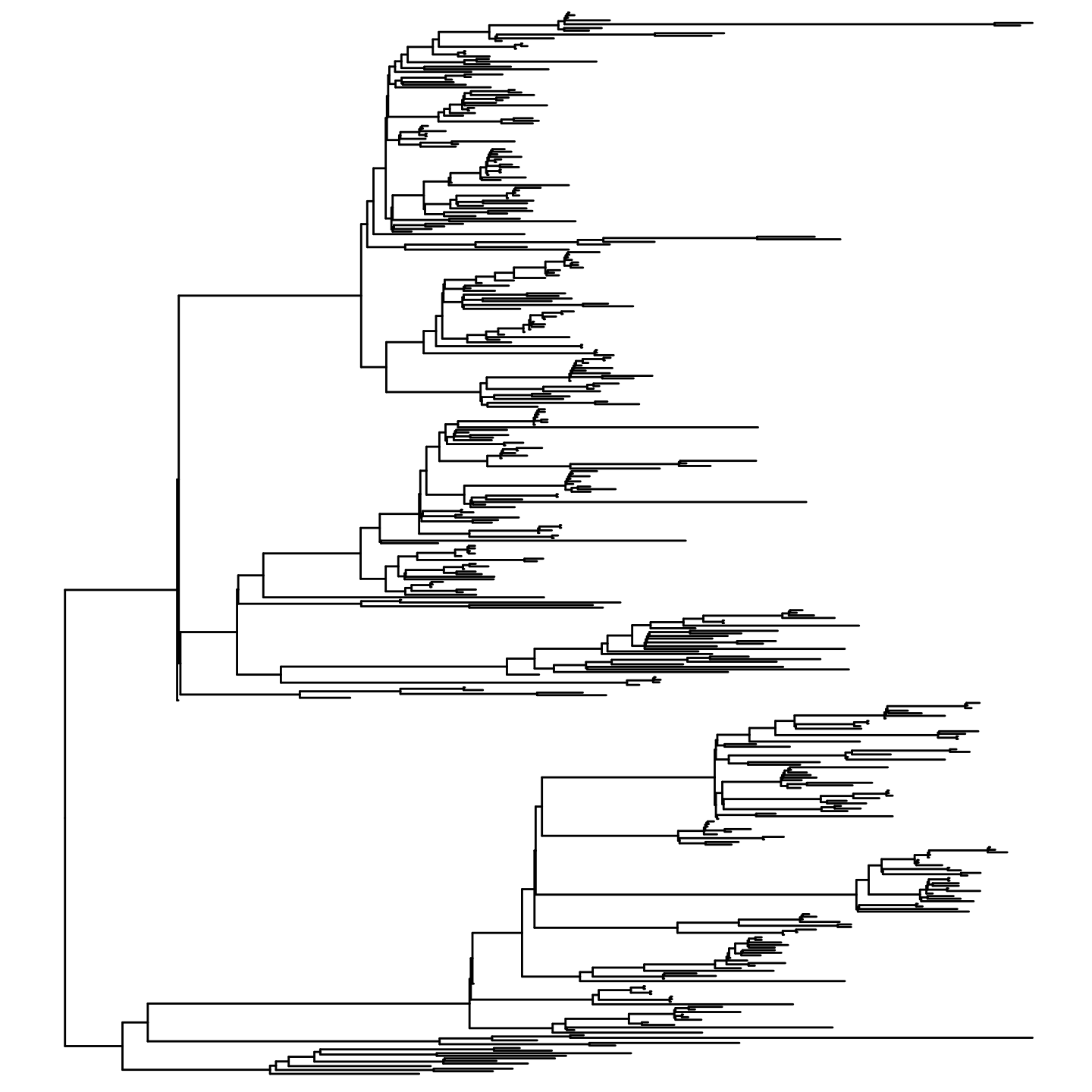
Step 0: Visualization of the trait across the phylogenetic tree
Before performing ancestral state reconstruction, it is critical to visualize the tip states of the trait on the phylogeny.
Our ancestral state reconstruction and clustering algorithm is most powerful in settings where frequent emergence and spread of a trait occurs.
Notice the clustering of Colistin non-susceptibility across the phylogeny.
Numerous emergence events at ancestral nodes and tips can be visually inferred in this phylogeny
Ancestral emergence events had noticeable variations in size. For instance, consider the large cluster of non-susceptibility in the above clade
feature_colors <- c(`1` = "black",`0`="white")
feature_scale <- ggplot2::scale_fill_manual(values=feature_colors,labels=c("Present","Absent"),name="Tip State", guide = guide_legend(nrow=1, title.position = "top", label.position = "right"))

p0 <- ggtree::gheatmap(ggtree::ggtree(tr),df %>% as.data.frame %>% select(colistin_ns) %>% mutate_all(as.factor),colnames_position = 'top',width = .25,low = 'white',high='black',colnames_angle = 90,legend_title = 'Colistin non-susceptibility',hjust = 0,color = NULL) + ylim(NA,485) + feature_scale
#> Scale for y is already present.
#> Adding another scale for y, which will replace the existing scale.
#> Scale for fill is already present.
#> Adding another scale for fill, which will replace the existing scale.
p0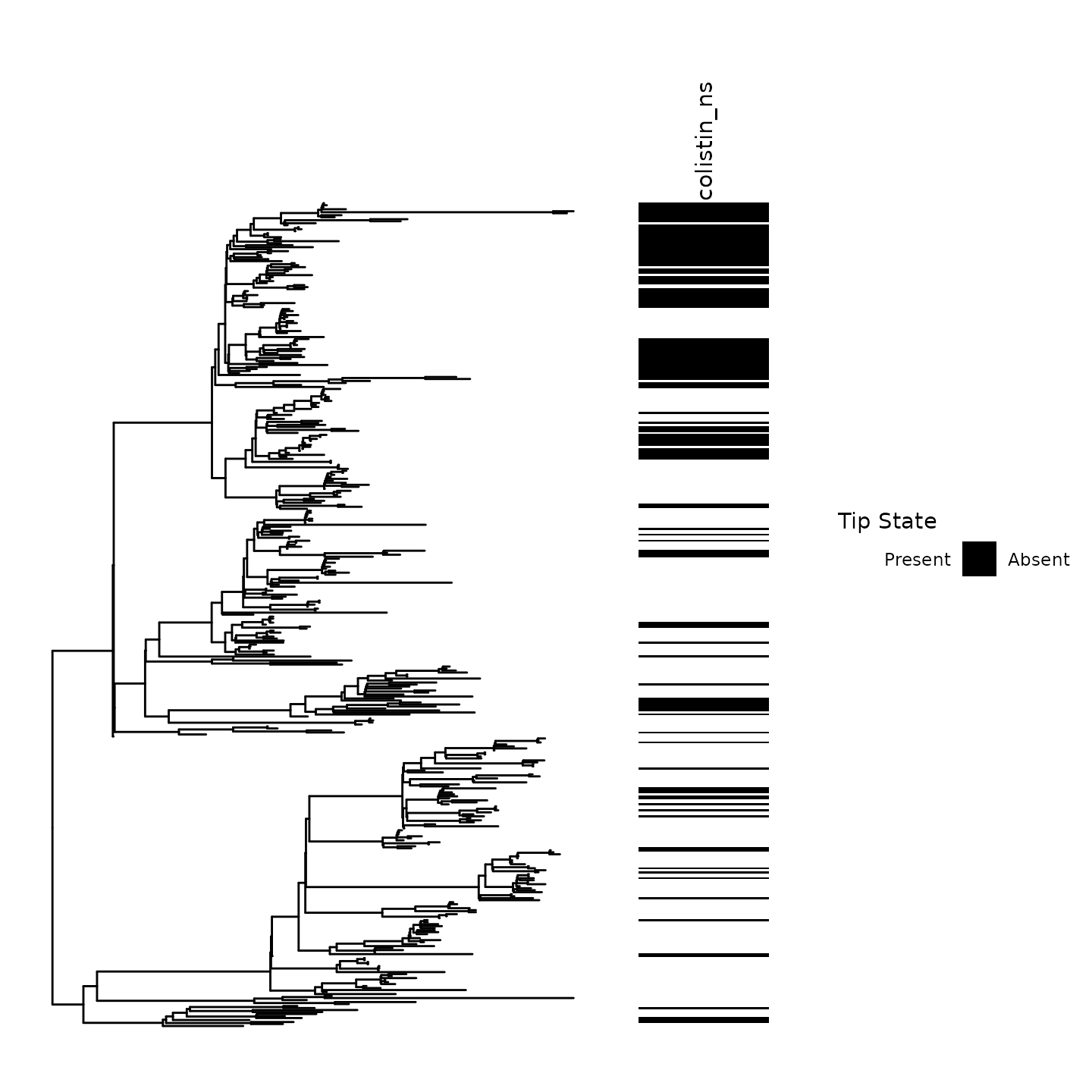
Step 1: Run ancestral state reconstruction
The workhorse function, asr(), is used to perform ancestral state reconstruction. This wrapper function implements ancestral state reconstruction with a single rate category using the corHMM R package: https://github.com/thej022214/corHMM
Using inferred ancestral states and tip-based data, edges on the phylogenetic tree were evaluated to determine episodes where the trait continued (i.e., susceptible -> susceptible or non-susceptible -> non-susceptible), was gained (i.e., susceptible -> non-susceptible), or was lost (i.e., non-susceptible -> susceptible). This edge matrix can be leveraged for numerous applications, including characterizing the frequency of trait transitions across a phylogeny and investigating phenotype-genotype associations.
-
The following parameters exist for this function
df: Dataframe with tip name variable (e.g., tip_name_variable) and trait variable (e.g., colistin_ns)
tr: Phylogenetic tree object of class phylo
-
model: This approach permits the use of either the equal rates (ER) or the all rates differ (ARD) transition matrices.
Equal rates: Assumes equal transition rates for trait gain (e.g., trait absence -> presence) or loss (e.g., trait gain -> absence)
All rates differ: Assumes different transition rates for trait gain and loss
-
node_states: Whether to perform ‘joint’ or ‘marginal’ ancestral state reconstruction
- From our experience, we recommend using joint ancestral state reconstruction.
Aside: Determining the best model
While we suggest the use of the equal rates (ER) transition matrix as the chosen model for corHMM, some instances permit the modeling of a trait using the all rates differ (ARD) model.
We implemented a function called, find_best_asr_model(), which performs ancestral state reconstruction using both the ER and ARD model.
Next, the best model is chosen using the Akaike information criteria (AIC). Specifically, the model with the lowest AIC is chosen.
The asr() function has the option to run this model finding algorithm using the model = “MF” argument.
best_model_obj <- phyloAMR::find_best_asr_model(df = df,tr = tr,tip_name_variable = "tip_name_var",trait = 'colistin_ns',node_states = 'joint')
#> Testing equal rates (ER) model
#> You specified 'fixed.nodes=FALSE' but included a phy object with node labels. These node labels have been removed.
#> State distribution in data:
#> States:  0   1
#> Counts:  277 136
#> Beginning thorough optimization search -- performing 0 random restarts
#> Finished. Inferring ancestral states using joint reconstruction.
#> AICc of ER model is: 357.950996595162
#> Testing all rates differ (ARD) model
#> You specified 'fixed.nodes=FALSE' but included a phy object with node labels. These node labels have been removed.
#> State distribution in data:
#> States:  0   1
#> Counts:  277 136
#> Beginning thorough optimization search -- performing 0 random restarts
#> Finished. Inferring ancestral states using joint reconstruction.
#> AICc of ARD model is: 355.966418109559
#> Best model: ARD

paste0("Model fit statistics: ")
#> [1] "Model fit statistics: "
best_model_obj$model_options
#> NULL

paste0("Best model: ")
#> [1] "Best model: "
best_model_obj$best_model
#> [1] "ARD"
Running ancestral state reconstruction
asr_obj <- phyloAMR::asr(df = df,tr = tr,tip_name_variable = "tip_name_var",trait = "colistin_ns",model = "ER",node_states = "joint")
#> You specified 'fixed.nodes=FALSE' but included a phy object with node labels. These node labels have been removed.
#> State distribution in data:
#> States:  0   1
#> Counts:  277 136
#> Beginning thorough optimization search -- performing 0 random restarts
#> Finished. Inferring ancestral states using joint reconstruction.

paste0("Output names: ")
#> [1] "Output names: "
names(asr_obj)
#> [1] "corHMM_output"           "corHMM_model_statistics"
#> [3] "parent_child_df"         "node_states"

paste0("corHMM_out: output from ancestral state reconstruction algorithm hosted in the R package corHMM")
#> [1] "corHMM_out: output from ancestral state reconstruction algorithm hosted in the R package corHMM"
asr_obj$corHMM_out
#>
#> Fit
#>        lnL      AIC    AICc Rate.cat ntax
#>  -177.9706 357.9413 357.951        1  413
#>
#> Legend
#> [1] "colistin_ns"
#> [1] "0" "1"
#>
#> Rates
#>          0        1
#> 0       NA 89553.08
#> 1 89553.08       NA
#>
#> Arrived at a reliable solution

paste0("corHMM_model_summary: A summary of the corHMM model, including the number of parameters, model, number of rate categories, inferred transition rates, log likelihood, AIC, and AICc")
#> [1] "corHMM_model_summary: A summary of the corHMM model, including the number of parameters, model, number of rate categories, inferred transition rates, log likelihood, AIC, and AICc"
paste0("Rate 1 = transitions from level 1 (i.e., susceptible) to level 2 (i.e., non-susceptible)")
#> [1] "Rate 1 = transitions from level 1 (i.e., susceptible) to level 2 (i.e., non-susceptible)"
paste0("Rate 2 = transitions from level 2 (i.e., non-susceptible) to level 1 (i.e., susceptible)")
#> [1] "Rate 2 = transitions from level 2 (i.e., non-susceptible) to level 1 (i.e., susceptible)"
asr_obj$corHMM_model_summary
#> NULL

paste0("node_states: Chosen node state that was modeled.")
#> [1] "node_states: Chosen node state that was modeled."
asr_obj$node_states
#> [1] "joint"

paste0("parent_child_df: Parent child dataframe, which contains the edge dataset, parent and child values, the child name (for tips), and transition data (i.e., gain, loss, and continuation of the trait on tree or continuation of trait absence on tree)")
#> [1] "parent_child_df: Parent child dataframe, which contains the edge dataset, parent and child values, the child name (for tips), and transition data (i.e., gain, loss, and continuation of the trait on tree or continuation of trait absence on tree)"
head(asr_obj$parent_child_df)
#>   parent child parent_value child_value child_name transition gain loss
#> 1    414   415            0           0       <NA>          0    0    0
#> 2    415   416            0           0       <NA>          0    0    0
#> 3    416   417            0           0       <NA>          0    0    0
#> 4    417   418            0           1       <NA>          1    1    0
#> 5    418   419            1           1       <NA>          0    0    0
#> 6    419   420            1           1       <NA>          0    0    0
#>   continuation continuation_present continuation_absent
#> 1            1                    0                   1
#> 2            1                    0                   1
#> 3            1                    0                   1
#> 4            0                    0                   0
#> 5            1                    1                   0
#> 6            1                    1                   0
Step 2: Describe the model (e.g., rates and fit)
The function, characterize_asr_model(), can be leveraged on corHMM output to identify the inferred rates and model fit statistics (i.e., log likelihood and AIC values)
phyloAMR::characterize_asr_model(asr_obj$corHMM_out)
#>   model number_parameters number_rate_categories    rate1 rate2    loglik
#> 1    ER                 1                      1 89553.08    NA -177.9706
#>        AIC    AICc
#> 1 357.9413 357.951
Step 3: Characterize the transition statistics for the trait across the phylogeny
The frequency and location of trait gain, loss, and continuation events can be characterized using the asr_transition_analysis() function
In this case, several important observations occur:
- Of 824 edges, 48 contained transition events: 37 gain events and 11 loss events
- Inference of location of these transition events revealed numerous
events at the tips:
- 30/37 gain events
- 7/11 loss events
- The number of gain events and large number of non-susceptible
isolates not accounted for by gain events at the tip, suggest potential
for inferred gain events to be shared across isolates.
- This is indicative of the emergence and spread of colistin non-susceptible strains in this population
- We also provide frequency statistics for the gain, loss, and continuation of these traits that can be useful to characterize the transition dynamics of this trait:
asr_transition_analysis(asr_obj$parent_child_df,node_states='joint')
#>   total_edges transitions gains gains_tip losses losses_tip continuations
#> 1         824          48    38        31     10          7           776
#>   continuations_present continuations_absent gain_frequency loss_frequency
#> 1                   206                  570           6.25           4.63
#>   continuation_present_frequency continuation_absent_frequency
#> 1                             25                         69.17
Step 4: Visualize the states on the phylogeny
Paint the tree
painted_tree <- phyloAMR::paint_tree_with_states(asr_obj$parent_child_df,tr)
#> Joining with `by = join_by(node)`
painted_tree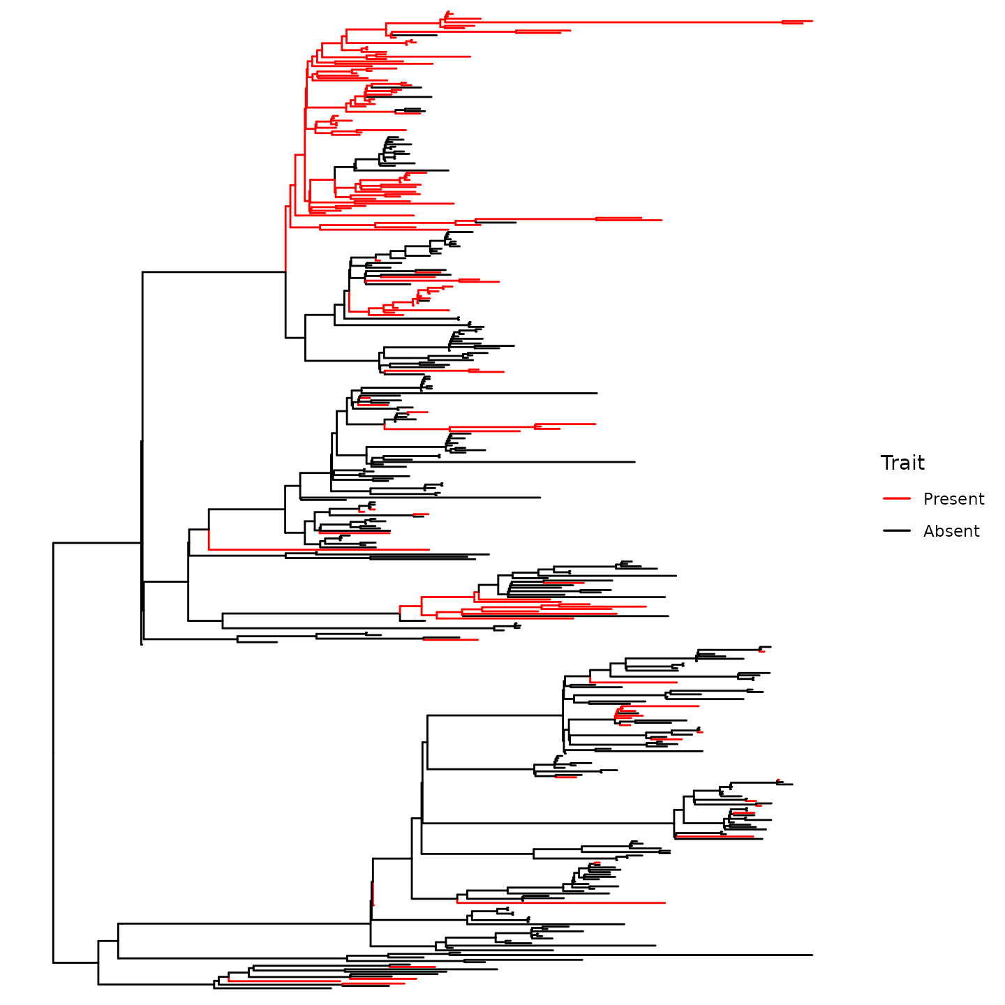
What’s next?
This algorithm can be leveraged to ask numerous questions. Specifically, we build the following functions to address questions of interest:
| Do isolates belong to episodes of trait emergence or spread? | asr() + asr_cluster_detection() + asr_cluster_analysis() |
| Genetic features associated with trait/lineage emergence/spread? | asr() + synchronous_detection() + synchronous_permutation_test() |
| What genotypes are subsequently gained/lost upon acquisition of a trait (i.e., potential compensatory or revertant mutations) | asr() + downstream_gain_loss() + downstream_permutation_test() |
| What descriptive characteristics are associated with phenotypic emergence and spread? | phyloaware_regression() |